Chapter 24: ML Systems & AI Infrastructure

Machine learning systems are software systems with an additional dimension of complexity: the behavior of the system is determined not only by code, but by data and model weights that evolve over time. Building reliable ML systems requires applying the full discipline of software engineering — versioning, testing, monitoring, deployment automation — to artifacts that most software engineers have never had to version before: datasets, feature pipelines, and trained model files.

---

Mind Map

---

The ML System Landscape

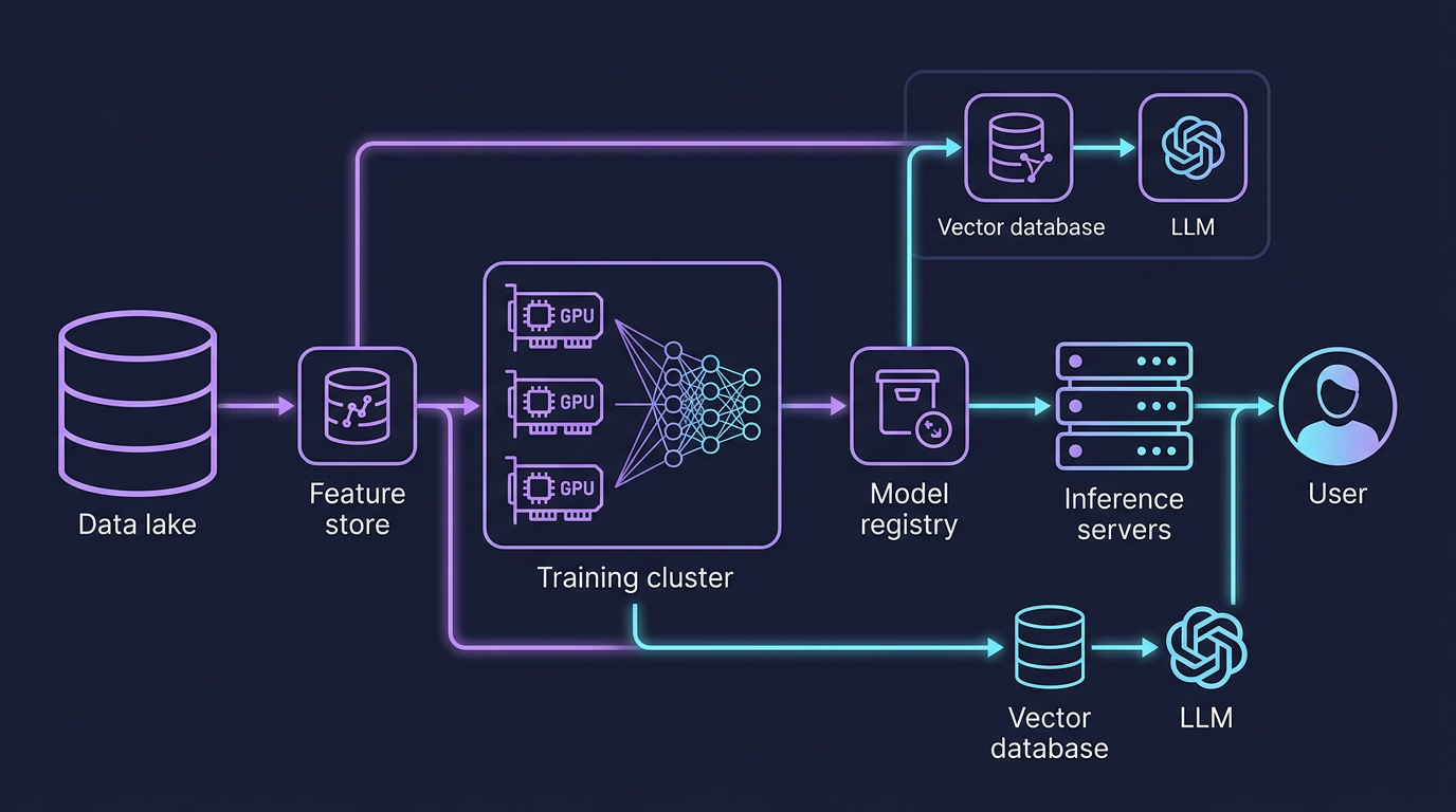
A production ML system is not a Jupyter notebook deployed as a Flask app. It is a complex sociotechnical system spanning data engineering, distributed computing, model development, and operational infrastructure. Google's landmark paper "Machine Learning: The High-Interest Credit Card of Technical Debt" identified the core challenge: ML code is typically a small fraction of a production ML system — the surrounding infrastructure for data collection, feature computation, model serving, monitoring, and configuration management is far larger and harder to maintain.

The five phases of every ML pipeline:

1. Data Collection — Ingest raw signals: user events, sensor readings, labels from human annotators
2. Feature Engineering — Transform raw data into numerical representations suitable for models
3. Training — Optimize model weights on historical data; potentially distributed across many Graphics Processing Units (GPUs)
4. Evaluation — Validate model quality on held-out data; run A/B tests in production
5. Serving — Deploy the model to make predictions on live traffic; batch or real-time

---

Feature Stores

Why Feature Stores Exist

The central problem feature stores solve is the training-serving skew: features computed during training must be computed identically during serving. Without a shared abstraction, ML teams reimplement the same feature logic in Python (training) and Java or Go (serving) — two codebases that inevitably diverge, silently degrading model accuracy.

A second problem is feature reuse. Across a large organization, dozens of teams independently compute "user's average purchase amount over the last 30 days." Without a shared store, each team writes, tests, and maintains their own version, often with subtle differences.

The third problem is point-in-time correctness. Training data must reflect the feature values that existed at the moment a label was generated — not the current values. A feature store with time-travel semantics prevents data leakage, where future information contaminates training labels.

Feature Store Architecture

Feast vs Tecton (now Databricks Feature Store)

Note: Tecton was acquired by Databricks and is now integrated into the Databricks platform. The comparison below reflects Tecton's capabilities as incorporated into Databricks.

Dimension	Feast	Tecton / Databricks Feature Store
Type	Open-source	Managed SaaS (Databricks platform)
Deployment	Self-hosted on any cloud	AWS, GCP, Azure — managed by Databricks
Online store	Redis, DynamoDB, Bigtable	Managed DynamoDB / Databricks-native
Offline store	S3, GCS, BigQuery, Snowflake	Delta Lake, S3, Snowflake
Streaming support	Via Kafka + custom jobs	Native Spark Structured Streaming
Point-in-time joins	Yes (offline only)	Yes (offline + backfills)
Transformation engine	External (user brings Spark/dbt)	Built-in Spark + managed pipelines
Best for	Teams wanting full control, budget-conscious	Large enterprises, Databricks ecosystem
Operational overhead	High — you run Redis, Spark, registry	Low — fully managed stack

Design rule: Use a feature store when: (a) more than one model uses the same feature, (b) features are expensive to compute (aggregations over billions of rows), or (c) the training-serving gap has caused accuracy regressions in production. For a single-model prototype, a feature store is premature.

---

Training Infrastructure

Distributed Training Strategies

Single-GPU training hits a wall on two dimensions: memory (a model must fit in GPU VRAM) and throughput (one GPU can only process so many examples per second). Distributed training solves both by spreading computation across many GPUs, often across many machines.

Three parallelism strategies:

Strategy	What is split	When to use	Communication overhead
Data parallelism	Mini-batch split across GPUs; each GPU has full model copy	Model fits in one GPU; need throughput	AllReduce gradient sync each step — O(params)
Model parallelism	Model layers split across GPUs	Model too large for one GPU (LLMs, >7B params)	Activation tensors passed between GPUs each layer
Pipeline parallelism	Layers split; mini-batches pipelined through stages	LLMs + large batch sizes	Micro-batch bubbles between stages
Tensor parallelism	Individual weight matrices split across GPUs	Very large transformer layers	Requires high-bandwidth interconnect (NVLink)

GPU Cluster Architecture

Within-node vs. across-node communication is a critical design constraint. NVLink between GPUs on the same node is ~600 GB/s. InfiniBand between nodes is ~400 Gb/s (50 GB/s) — roughly 12x slower. Training frameworks (PyTorch FSDP, DeepSpeed) are designed to minimize cross-node gradient communication by preferring data locality.

Parameter servers (an older pattern) used a centralized server to aggregate gradients. Modern training uses AllReduce (ring-based or tree-based) to aggregate gradients peer-to-peer without a bottleneck server. NCCL (NVIDIA Collective Communications Library) implements AllReduce optimized for GPU interconnects.

---

Model Serving: Batch vs Real-Time

Serving is where the model generates business value. The serving architecture — batch or real-time — is determined by latency requirements, throughput, and the nature of the use case.

Dimension	Batch Inference	Real-Time Inference
Latency	Hours to days (scheduled jobs)	Milliseconds (P99 < 100ms typical)
Throughput	Millions to billions of examples per run	Hundreds to thousands of QPS
Trigger	Schedule (nightly), event (bulk upload)	User request
Infrastructure	Spark, Ray, Kubernetes Jobs	TF Serving, Triton, vLLM, SageMaker
GPU utilization	Near 100% (large batches maximize GPU efficiency)	Often 20–60% (small batches from live traffic)
Cost	Low cost/prediction (high utilization)	Higher cost/prediction (idle capacity needed for latency SLA)
Feature freshness	Features from offline store (hours old)	Features from online store (seconds old)
Error handling	Retry job; re-run failed partitions	Fallback model, default value, circuit breaker
Use cases	Recommendation pre-computation, churn scoring, fraud scoring on past transactions	Search ranking, fraud detection on live payment, NLP response generation
Output storage	Written back to data warehouse / KV store	Returned in API response

Decision rule: When you can pre-compute predictions for a known set of entities (all users, all products), batch inference is cheaper and simpler. When the prediction must incorporate events that just happened (user's last click, real-time transaction amount), real-time inference is required.

---

Model Serving Architectures

Overview

TF Serving is Google's production server for TensorFlow SavedModels. It supports server-side request batching (accumulates requests for up to N milliseconds and processes them as a single batch, increasing GPU utilization), model versioning with hot-swap (load a new model version without restart), and REST + gRPC protocols.

Triton Inference Server (NVIDIA) is framework-agnostic: it serves TensorFlow, PyTorch, ONNX, and TensorRT models from the same binary. Its key differentiator is the backend plugin system — custom backends can handle arbitrary computation. Triton's dynamic batching scheduler automatically combines concurrent requests into a single GPU call.

vLLM is purpose-built for large language models. Its breakthrough innovation is PagedAttention: KV cache memory is managed in fixed-size pages (like OS virtual memory paging), enabling serving many more concurrent requests than naive per-request KV cache allocation allows. It also implements continuous batching — new requests join a running batch as soon as a slot frees, rather than waiting for the entire batch to complete.

SageMaker Endpoints abstract all infrastructure: you upload a model artifact to S3, define an endpoint configuration (instance type, auto-scaling policy), and AWS manages model loading, health checks, traffic routing, and scaling. The trade-off is less control and higher cost per inference versus self-hosted Triton.

---

LLM Inference & Serving (2026)

Large language model (LLM) inference has its own serving stack that is architecturally different from traditional ML model serving. The core challenge: LLMs generate tokens autoregressively (one at a time), hold large KV caches in GPU memory, and exhibit highly variable output lengths — none of which traditional serving frameworks (TF Serving, Triton) were designed for.

The Inference Framework Landscape

As of 2026, the LLM serving framework landscape has converged:

Framework	Status	Key Innovation	Best For
vLLM	De facto production standard	PagedAttention (virtual KV cache paging); continuous batching; OpenAI-compatible API	Most production deployments; open-source and self-hosted
SGLang	Strong alternative	RadixAttention (tree-based KV cache reuse for shared prefixes); structured output generation	Long system prompts shared across requests; constrained generation (JSON schema)
TensorRT-LLM	NVIDIA-specific, high performance	FP8 quantization on H100/H200; kernel fusion; INT8/INT4	Maximum throughput on NVIDIA hardware; requires NVIDIA ecosystem
HF TGI (Text Generation Inference)	Maintenance mode since Dec 2025	Was widely used; now only receiving bug fixes	Legacy deployments; HF Inference Endpoints now default to vLLM
Ollama	Local/edge deployment	Easy single-machine deployment; quantized models	Development; local inference; small-team deployment

TGI Maintenance Status

Hugging Face Text Generation Inference (TGI) entered maintenance mode in December 2025 — it accepts only bug fixes, no new features. For new deployments, use vLLM or SGLang. Hugging Face's own Inference Endpoints now default to vLLM.

GPU utilization comparison: vLLM achieves 85–92% GPU utilization vs TGI's 68–74% due to more efficient KV cache management. This directly translates to cost: the same GPU fleet serves significantly more traffic under vLLM.

PagedAttention: Virtual Memory for KV Cache

The key bottleneck in LLM serving is KV cache memory management. During autoregressive generation, each token in the context window requires Key and Value tensors to be stored for every attention head in every layer. For a 70B parameter model with a 4K token context, this can be tens of gigabytes per request.

Traditional serving allocates a contiguous memory block for each request's KV cache upfront — based on the maximum possible output length. This wastes most of the allocation (most responses are shorter than the max) and severely limits how many requests can be served concurrently.

PagedAttention (vLLM's core innovation) applies the OS virtual memory paging concept to KV cache: physical GPU memory is divided into fixed-size pages, and each request gets pages allocated on demand as tokens are generated. Pages from completed requests are immediately freed for reuse. The result: near-zero KV cache fragmentation, 2–4× more concurrent requests on the same GPU, and no upfront over-allocation.

Continuous Batching (In-Flight Batching)

Static batching waits for a full batch of requests, processes all of them, returns all results, then accepts the next batch. This causes GPU idle time whenever requests in the batch finish at different times (which is always — LLM output lengths vary enormously).

Continuous batching (also called in-flight batching) inserts new requests into the running batch as soon as existing requests complete their generation. The GPU is never idle waiting for a batch to finish.

Combined impact of PagedAttention + continuous batching: GPU utilization rises from ~30% (naive static batching) to ~80–90%, directly multiplying effective throughput without additional hardware.

Speculative Decoding

LLM decoding is memory-bandwidth bound, not compute bound — at inference time, the GPU spends most of its time loading model weights from HBM (high bandwidth memory), not performing matrix multiplications. This means much of the GPU's compute capacity is idle during single-request generation.

Speculative decoding exploits this idle compute by running a small draft model (e.g., a 1B parameter model) in parallel with the large target model (e.g., 70B). The draft model rapidly proposes K tokens; the target model verifies all K proposed tokens in a single parallel forward pass. If all K are accepted, K tokens are generated for the cost of approximately one target model step.

Real-world throughput gains: 2–3.87× token generation speed without any change in output quality (the target model's distribution is preserved exactly). Speculative decoding is now standard in vLLM, SGLang, and TensorRT-LLM — not a research technique.

Practical requirements:

• Draft and target models must share tokenizer and output vocabulary
• Best gains when the draft model acceptance rate is > 70% (domain-matched drafts help)
• Requires enough GPU memory for both models simultaneously

Quantization for LLM Inference

The quantization table in the GPU Optimization section above covers formats. For LLMs specifically, 2026 best practices:

• FP8 on H100/H200: FP8 (8-bit floating point) is the sweet spot on H100/H200 hardware — near-FP16 accuracy with 2× throughput and half the memory bandwidth pressure. TensorRT-LLM and vLLM both support FP8.
• GPTQ / AWQ (INT4): Calibrated 4-bit quantization that minimizes accuracy loss vs naive INT4. A 70B model fits on a single 40GB A100 in INT4. Accuracy loss is 1–3% on most benchmarks for modern calibration methods.
• KV cache quantization (INT8): Separate from weight quantization — quantizing only the KV cache to INT8 reduces its memory footprint by 2× with minimal accuracy impact, allowing more concurrent requests at full weight precision.

Disaggregated Prefill and Decode

A 2025–2026 production pattern for very large deployments: disaggregating the prefill and decode phases onto separate GPU pools.

• Prefill (processing the full input prompt) is compute-intensive but fast: runs once, parallelizes well
• Decode (generating output tokens one at a time) is memory-bandwidth-bound and latency-sensitive

Running both on the same GPU cluster means prefill bursts interfere with decode latency, causing P99 spikes. Disaggregation routes prefill to a separate pool of GPUs optimized for compute throughput, and decode to a pool optimized for memory bandwidth and latency. The KV cache is transferred between pools after prefill completes.

This pattern is emerging in hyperscaler deployments (Google, Meta, large cloud providers) and is supported by llm-d and experimental vLLM disaggregation features. At most organization scales, a single pool with careful batching is sufficient.

---

RAG Architecture: Production Patterns

The RAG Architecture section above introduces the concept. This section deepens the production engineering perspective, covering the decisions that most affect retrieval quality and system performance.

Chunking Strategy: The Biggest Quality Lever

Chunking is underestimated. Poor chunking degrades RAG accuracy more than model choice, embedding model choice, or retrieval algorithm choice. The goal: chunks should be semantically coherent, self-contained enough to be useful in isolation, and sized to match your embedding model's effective context window.

Strategy	How It Works	Best For	Trade-off
Fixed-size with overlap	Split every N tokens; overlap K tokens between chunks	Simple baseline; most document types	May split mid-sentence, breaking context
Recursive character splitter	Split on paragraph → sentence → word boundaries, respecting structure	Code, prose; general purpose	Slightly more complex, better coherence
Document-structure-aware	Split on Markdown headers, HTML tags, PDF section boundaries	Technical docs, wikis, structured content	Requires document type detection
Semantic chunking	Use embedding similarity to detect topic shifts; split at low-similarity boundaries	Research papers, long-form content	Computationally expensive; slower ingestion
Hierarchical / parent-child	Store large parent chunks; retrieve small child chunks; inject parent context into LLM	When context around a fact matters	More index complexity; two retrieval steps

Rule of thumb: Start with a recursive character splitter at 512 tokens with 50-token overlap. Measure retrieval recall on a sample query set. If recall is low, try semantic chunking or document-structure-aware splitting.

Full Production RAG Pipeline

Two-stage retrieval is standard: Stage 1 (ANN search, top-50) optimizes recall. Stage 2 (cross-encoder reranker, top-5) optimizes precision. The reranker sees both query and document jointly — more accurate than cosine similarity, which embeds them independently.

Hybrid retrieval beats pure vector search on most production benchmarks. BM25 (sparse keyword matching) catches exact-match queries that dense retrieval misses (product codes, proper nouns, rare terms). Weaviate and Elasticsearch natively support hybrid search; pgvector can combine with ts_vector full-text for similar effect.

Agentic RAG and Advanced Patterns

Beyond the baseline retrieval-generation pipeline, 2026 production systems use:

Graph RAG: Builds a knowledge graph from the document corpus. Entities and relationships are extracted and stored as graph edges. Retrieval traverses the graph rather than performing pure vector search — effective when the answer requires connecting multiple facts across documents (e.g., "What are all the projects that depend on library X which has vulnerability Y?").

Multi-hop RAG: The LLM generates sub-questions, retrieves for each sub-question, synthesizes partial answers, then generates the final answer. More accurate for complex questions requiring multiple reasoning steps. Slower and more expensive.

RAG evaluation: Track retrieval recall (are the relevant chunks in the top-K?), context precision (are retrieved chunks actually relevant?), and answer faithfulness (does the answer actually come from the retrieved context?). Tools: RAGAS, TruLens, LangSmith.

---

LLM Gateways, Routing & Semantic Caching

As organizations move from a single LLM API to a portfolio of models (internal, cloud-hosted, specialized), an LLM gateway becomes essential infrastructure — the same role that an API gateway plays for microservices.

What an LLM Gateway Provides

LiteLLM is the most widely adopted open-source gateway (2026): unified OpenAI-compatible API across 100+ providers, with built-in cost tracking, rate limiting, and basic routing. For enterprises, custom gateways built on LiteLLM or llm-d add cache-aware routing.

Semantic Caching

Traditional caching matches requests exactly — the same byte sequence returns the same cached response. Semantic caching matches by meaning: if a user asks "What is the capital of France?" and the cache contains "Tell me the capital city of France?", the semantic cache returns the same cached answer without calling the LLM.

Production impact:

• Typical cache hit rates: 40–60% for enterprise internal tools (users ask similar questions repeatedly)
• Cost reduction: 30–80% depending on query diversity and cache size
• Latency improvement: cache hits return in < 50 ms vs 500 ms – 10 s for LLM inference

Threshold tuning: The similarity threshold determines precision vs recall of cache hits. At 0.95 cosine similarity, only near-identical queries hit the cache. At 0.85, more hits but occasional wrong-answer cache returns. Typical production values: 0.90–0.93.

Layered caching strategy:

1. Exact match cache (Redis, hash of request): sub-millisecond; handles identical repeated queries
2. Semantic cache (vector similarity): 10–50 ms lookup; handles paraphrased queries
3. Provider-level cache (OpenAI prompt caching): 50% discount on repeated prompt prefixes; free, automatic

Intelligent Model Routing

Beyond load balancing, intelligent routing selects the optimal model for each request based on:

Routing Signal	How It Works	Example
Task classification	Classify query type (code / chat / extraction / reasoning)	Route code queries to a code-specialized model
Cost optimization	Route simple queries to cheaper models	Single-hop factual questions → Haiku; complex reasoning → GPT-4o
Latency SLA	Route latency-sensitive paths to fastest model	Realtime chatbot → fast model; background summarization → slow cheaper model
KV cache utilization	Route to the instance with the longest shared prefix in cache	108% throughput improvement possible with cache-aware routing
Fallback	Primary model unavailable / rate-limited → secondary	GPT-4o down → Claude Sonnet

Cache-aware routing is a 2025–2026 advance: instead of round-robining across vLLM instances, route each request to the instance that already has the longest matching prefix in its KV cache (prefix caching / prompt caching). This dramatically increases prefix cache hit rates — especially for RAG workloads where system prompts and retrieved context are repeated across many requests.

---

Architecting Agentic AI Systems

Agentic AI systems extend LLMs from single-turn question answering into multi-step autonomous workflows. An agent perceives input, calls tools, reasons about results, and takes further actions — potentially over many iterations — to accomplish a goal.

Anatomy of an Agent

Tool / function calling is the mechanism by which LLMs interact with the external world. The LLM generates a structured JSON call specifying tool name and arguments; the runtime executes the tool and returns the result as the next input. OpenAI-compatible function calling is now standard across all major LLM APIs.

Orchestration Frameworks (2026)

Framework	Architecture	Strengths	Caution
LangGraph	State machine / DAG of nodes	Explicit control flow; human-in-the-loop; streaming; persistence	More boilerplate than simple agents
AutoGen (Microsoft)	Multi-agent conversation	Natural multi-agent patterns; code execution built-in	Less explicit state control
CrewAI	Role-based multi-agent	Fast to set up; role definitions are intuitive	Less flexible for complex graphs
Direct API (no framework)	Plain function calls + loop	Full control; minimal abstraction overhead	More implementation work

LangGraph is the most production-adopted framework for complex agents in 2026 — it models agent execution as a directed graph of nodes (LLM calls, tool calls, conditional branches) with persistent state at each node. This makes human-in-the-loop (pause execution for user approval), streaming, and checkpointing natural.

Memory Architecture

Agents need memory across two dimensions:

Short-term memory = context window. The active conversation, current task state, and tool outputs are all part of the LLM's prompt context. Context window management (what to include, what to summarize or truncate) is critical — a 128K context window sounds large but fills quickly in multi-step agents.

Long-term memory = vector retrieval. Relevant past interactions and stored facts are retrieved from a vector store and injected into the context at each turn. This gives agents persistent "memory" without relying on a finite context window.

Multi-Agent Systems

Complex tasks benefit from specialization: rather than one all-purpose agent, use a network of specialized agents with defined roles.

Key design patterns:

• Orchestrator / worker: One agent decomposes tasks and delegates; workers execute and return results
• Peer collaboration: Agents critique each other's outputs iteratively (debate pattern)
• Validation loop: A reviewer agent checks each worker's output before passing to the next stage

Reliability concern: In multi-agent systems, errors compound. An agent that misunderstands a subtask propagates that misunderstanding to subsequent steps. Define clear interfaces between agents; add explicit validation checkpoints.

Guardrails, Safety & Evaluation

Agentic systems introduce new reliability and safety concerns not present in single-turn LLM calls:

Input guardrails: Detect prompt injection (malicious instructions embedded in retrieved documents or user input that attempt to hijack the agent); scope the agent to its intended domain; filter PII before it enters the LLM.

Output guardrails: Check that factual claims are grounded in retrieved context (faithfulness); filter harmful content; validate citations. Tools: Guardrails AI, NVIDIA NeMo Guardrails.

Tool execution guards: Limit what tools can do (read-only vs write permissions; scope to specific resources); require human confirmation for irreversible actions (deleting records, sending emails, making purchases); ensure rollback is possible.

Evaluation for agents is harder than for single-turn models — the right answer may be achieved through different tool call sequences, and errors may be subtle (a plausible but wrong intermediate step). Approaches:

• Trajectory evaluation: Score the sequence of tool calls, not just the final output
• LLM-as-judge: Use a stronger LLM to assess intermediate reasoning steps
• Unit test with mock tools: Test agent behavior on scripted tool response scenarios
• Tools: LangSmith, Braintrust, Promptfoo

Agentic AI Reliability (2026 State)

Agentic systems are powerful but not yet reliable enough for high-stakes autonomous operation without human oversight. As of 2026, the practical pattern is human-in-the-loop for consequential actions (any write operation, financial transaction, communication) and fully autonomous for read-only research and analysis tasks. Invest heavily in observability — log every agent step, every tool call, every LLM response — because debugging a multi-step agent failure without logs is nearly impossible.

---

MLOps: The ML Development Lifecycle

MLOps applies DevOps principles to machine learning: version everything, automate everything, monitor everything. The three pillars are experiment tracking, model registry, and Continuous Integration/Continuous Deployment (CI/CD) for ML.

Experiment Tracking

Every training run should be reproducible. Experiment trackers record the complete provenance of a model: hyperparameters, dataset version, code commit, environment, and resulting metrics.

MLflow is the open-source standard: mlflow.log_param(), mlflow.log_metric(), mlflow.log_artifact() instrument any Python training script. The MLflow UI shows runs side-by-side for comparison. Weights & Biases (W&B) is the managed alternative with richer visualization, team collaboration features, and deeper integration with PyTorch training loops.

Model Registry

A model registry is the deployment gatekeeper — it stores versioned model artifacts with metadata (metrics, dataset lineage, training config) and manages the promotion workflow from experimentation to production.

Promotion checklist before Production:

• Offline metrics exceed baseline (AUC, F1, RMSE depending on task)
• Shadow mode test: model runs in parallel without affecting users; predictions compared to production model
• Latency profiling: P99 < serving SLA under realistic concurrency
• Data validation: input feature distributions match training distribution

CI/CD for ML

Standard software CI/CD runs build + unit test + deploy. ML CI/CD adds data validation, model training, and model evaluation as pipeline stages.

Critical difference from software CI/CD: The "test" in ML CI is non-deterministic — two identical training runs on the same data can produce slightly different models due to random initialization, dropout, and floating-point nondeterminism. ML pipelines use relative evaluation (is this model better than the current production model?) rather than absolute assertions.

---

Vector Databases

Vector databases store high-dimensional embedding vectors and support Approximate Nearest Neighbor (ANN) search — finding the K vectors most similar to a query vector by cosine similarity or Euclidean distance. The "approximate" is intentional: exact nearest neighbor in high dimensions requires scanning all vectors, which is too slow at scale. ANN algorithms (HNSW, IVF) trade a small recall drop for orders-of-magnitude speed improvement.

How HNSW Works

Hierarchical Navigable Small World (HNSW) builds a multi-layer graph where each node is a vector. Upper layers are sparse (long-range connections), lower layers are dense (short-range). Search starts at the top layer, greedily navigates to the approximate region, then descends to the bottom layer for precise local search.

Vector Database Comparison

Dimension	Pinecone	Weaviate	pgvector
Type	Managed SaaS	Open-source + managed	Postgres extension
ANN algorithms	Proprietary (HNSW-based)	HNSW, flat	IVFFlat, HNSW
Deployment	Fully managed (no infra)	Self-hosted or Weaviate Cloud	Runs inside Postgres
Hybrid search	Metadata filters + vector	Vector + keyword (BM25) + filters	Vector + full SQL
Max scale	Billions of vectors	Billions (self-hosted)	Millions (Postgres limits)
Latency (10M vectors)	~10ms P99	~15ms P99 (self-hosted)	~50–200ms (depends on memory)
Multi-tenancy	Namespaces	Multi-tenancy built-in	Schema separation
Cost	Usage-based (free starter, paid from $50/month)	Infra cost + managed fees	Postgres instance cost
Best for	Production RAG, fast start	Open-source preference, hybrid search	Teams already on Postgres; <10M vectors
Weakness	Vendor lock-in; no raw index access	Operational complexity if self-hosted	Not designed for vector-first workloads

Decision framework:

• Already on Postgres with < 5M vectors → pgvector (zero new infrastructure)
• Need open-source with hybrid BM25 + vector search → Weaviate
• Need managed, fast time-to-production, > 100M vectors → Pinecone

---

GPU Optimization Techniques

GPU utilization in serving is often shockingly low — 20–40% is common for naive deployments. Three techniques dramatically improve throughput and reduce cost per inference.

Request Batching

A GPU's throughput is maximized when it processes many examples simultaneously (matrix multiplication efficiency scales with batch size). Real-time serving receives one request at a time, leaving GPU idle between requests.

Static batching: Wait up to N milliseconds for more requests to arrive, then process as a batch. Simple but adds fixed latency.

Continuous batching (for LLMs): Instead of waiting for all sequences in a batch to finish before accepting new requests, new requests are inserted into the batch dynamically as old sequences complete their generation. This is the breakthrough in vLLM: GPU utilization rises from ~30% to ~80%.

Quantization

Neural network weights are typically stored as 32-bit floats (FP32). Quantization reduces precision:

Format	Bits	Memory reduction	Accuracy impact	Use case
FP32	32	1× (baseline)	None	Training (full precision)
BF16	16	2×	Minimal (<0.1% quality drop)	Training + serving on A100/H100
FP16	16	2×	Minimal	Serving on older GPUs (V100)
INT8	8	4×	Small (0.5–2% accuracy drop)	High-throughput serving, cost-sensitive
INT4	4	8×	Moderate (2–5% for most tasks)	Edge devices, extreme cost savings
GPTQ / AWQ	4-bit	8×	Smaller than naive INT4	LLM serving — calibrated quantization

A 70B parameter LLM in FP32 requires 280 GB of GPU memory (70B × 4 bytes). In INT4, it requires 35 GB — fitting on a single 40GB A100. This is why quantization is essential for LLM deployment.

Model Parallelism for LLM Serving

KV Cache is a critical LLM inference optimization. During autoregressive text generation, each token's Key and Value matrices from the attention mechanism are cached so they don't need to be recomputed for subsequent tokens. Without KV cache, generating a 1000-token response requires recomputing attention over all previous tokens at every step — O(n²) computation. With KV cache, it is O(n). The cost: KV cache consumes significant GPU memory (vLLM's PagedAttention addresses this with virtual memory paging).

---

Deep Dive: How Netflix Serves ML Recommendations at Scale

Netflix generates hundreds of millions of personalized rankings daily — homepage rows, search results, notification targeting, and more. Their ML infrastructure represents one of the most sophisticated production ML systems publicly documented.

Scale

• ~300 million members, each with a unique ranking
• Hundreds of ML models in production simultaneously
• Billions of model predictions generated daily
• Latency SLA: homepage recommendations must load in under 200ms end-to-end

The Recommendation Architecture

The Two-Tower Model

Netflix uses a two-tower neural network architecture for candidate retrieval. One tower encodes the user (user embedding), the other encodes content (content embedding). Both produce vectors in the same embedding space. Candidate retrieval is then an ANN search: find the content embeddings nearest to the user embedding.

Key Engineering Decisions

Hybrid batch + real-time serving: Netflix precomputes candidate sets overnight (batch, cheap) but applies real-time ranking at request time (uses last-minute signals like "user just watched horror movie"). This separates the expensive retrieval problem (scale: all content × all users) from the latency-sensitive ranking problem (scale: 1000 candidates × current user).

EVCache for pre-computed candidates: Netflix built EVCache (Ephemeral Volatile Cache), a distributed memcached layer across AWS regions. Pre-computed candidate sets are written to EVCache after batch inference. At serving time, candidate retrieval is a single cache lookup with < 5ms P99 latency — no model inference required.

Paved road ML platform (Metaflow): Netflix open-sourced Metaflow, their Python framework for ML pipelines. It handles: versioned artifacts, compute resource allocation (local, AWS Batch, or Kubernetes), data access abstraction, and experiment reproducibility. Every Netflix ML model is built on Metaflow, so all models benefit from platform improvements automatically.

A/B testing infrastructure: Every new model is tested in an A/B experiment before promotion. Netflix's experimentation platform (XP) runs thousands of concurrent A/B tests. Model metrics (click-through rate, play rate, watch time) are computed in near-real-time using Flink streaming pipelines, enabling fast feedback on model quality.

Metric	Detail
Members	~300M globally
Candidate retrieval latency	< 5ms (EVCache hit)
End-to-end recommendation latency	< 200ms
Models in production	Hundreds simultaneously
Daily predictions	Billions
Retraining frequency	Daily for most models; hourly for some trend models
A/B tests running	Thousands concurrently

---

Key Takeaway

Building ML systems is 10% model training and 90% data, infrastructure, and operations. The model is the easy part — PyTorch and pretrained foundations have democratized training. The hard parts are: ensuring training and serving features are computed identically, maintaining reproducibility across hundreds of experiments, deploying models reliably with validation gates, detecting when models degrade silently as data distribution shifts, and serving predictions at millisecond latency under production traffic. Teams that invest in feature stores, experiment tracking, model registries, and monitoring infrastructure will iterate 10x faster than teams that treat each model as a one-off script. For LLMs specifically (2026), the production stack has converged: vLLM for inference (PagedAttention + continuous batching), RAG for grounding LLMs in private knowledge (with careful attention to chunking and reranking), semantic caching to cut LLM API costs 30–80%, and an LLM gateway for routing, observability, and fallback. Agentic systems are the next wave — powerful for research and automation tasks, but requiring investment in guardrails, tool scoping, and trajectory-level evaluation before autonomous deployment in production.

---

Related Chapters

Chapter	Relevance
Ch11 — Message Queues	Streaming data pipelines for real-time feature ingestion
Ch09 — SQL Databases	Feature store backed by SQL for training data retrieval
Ch23 — Cloud-Native	Kubernetes for GPU workloads and model serving infrastructure
Ch07 — Caching	Model prediction caching to reduce inference latency

---

Practice Questions

Beginner

1. Training-Serving Skew: Your fraud detection model achieves 0.92 AUC offline but only 0.78 AUC in production. Describe the three most likely causes of this gap (focusing on feature computation differences), and explain how a feature store would have prevented or detected each issue.

   Hint

   The three main causes: features computed differently at training time vs serving time, training data includes future information not available at inference (data leakage), and the production distribution has drifted from the training distribution — a feature store enforces identical computation for both.

Intermediate

2. RAG vs Fine-tuning: A legal tech company needs their LLM to answer questions over 500K internal case documents updated weekly. Compare RAG vs fine-tuning on: cost to build, cost to update when new cases are added, factual accuracy, hallucination risk, and query latency. Under what conditions would you recommend each approach?

   Hint

   Fine-tuning bakes knowledge into weights (expensive to update when documents change weekly); RAG retrieves from an index (cheap updates, add new docs to the vector store) but accuracy depends on retrieval quality — for frequently updated factual knowledge bases, RAG is almost always the right choice.

3. Vector Database Selection: You are building a knowledge management system for a 10,000-person enterprise with 50M document chunks. Requirements: vector similarity search, full-text keyword search, department/date filtering, and real-time updates. Your team already uses RDS Postgres extensively. Evaluate pgvector, Weaviate, and Pinecone for this use case and make a justified recommendation.

   Hint

   pgvector is the pragmatic choice for an existing Postgres shop (no new infrastructure, ACID guarantees, SQL filtering); its limitation is ANN performance at 50M vectors — acceptable if you accept slightly lower recall vs purpose-built vector DBs.

4. Distributed Training Design: Your team needs to train a 65B parameter transformer. A single H100 has 80GB VRAM; 65B params in BF16 requires 130GB. You have 16 nodes × 8 H100s. Specify which combination of data parallelism, tensor parallelism, and pipeline parallelism you would use, and identify the critical bottleneck in your design.

   Hint

   Use tensor parallelism within a node (split layers across 8 GPUs on shared NVLink) and pipeline parallelism across nodes (partition layers across nodes on InfiniBand); data parallelism across node groups — the critical bottleneck is inter-node bandwidth during gradient synchronization.

Advanced

5. LLM Serving Cost Optimization: Your customer support chatbot uses a 7B LLM: 4× A100 40GB (FP32), static batching, P99 800ms, 12 req/s throughput, $8K/month GPU cost. You need to cut cost by 60% while keeping P99 < 500ms and throughput > 30 req/s. Describe your optimization plan across quantization, batching strategy, and infrastructure. Estimate the impact of each change and verify all three constraints are met.

   Hint

   INT8 quantization halves GPU memory (can run on 2× A100 or smaller GPUs, -50% cost); continuous batching (vs static) increases GPU utilization and throughput 2–4×; switch to continuous batching framework (vLLM) — together these changes can achieve 60% cost reduction while improving throughput.

6. RAG System Design: Design a RAG system for a 50,000-person enterprise with a 10M-document internal knowledge base (policies, wikis, engineering docs, contracts). Requirements: P99 answer latency < 3s, support for hybrid keyword + semantic search, source citations in every answer, and the ability to add new documents in < 5 minutes. Specify the ingestion pipeline, chunking strategy, vector store selection, retrieval architecture, and how you handle stale cached answers when documents are updated.

   Hint

   Use document-structure-aware chunking (split on headers/sections); hybrid retrieval (Weaviate or pgvector + tsvector for BM25 + dense); two-stage retrieval (top-50 ANN → cross-encoder reranker → top-5); for freshness, use a document version hash: on document update, re-embed affected chunks and invalidate semantic cache entries by document ID. For 5-minute update SLA, run ingestion as a streaming pipeline (Kafka → chunker → embedder → vector store upsert) rather than batch.

7. Agentic System Design: Design an AI coding assistant that can read a codebase, write new code, run tests, debug failures, and open a pull request — with a human-in-the-loop checkpoint before the PR is submitted. Identify: the agent tools required, the memory architecture, where human approval gates should be placed, and the top three failure modes and their mitigations.

   Hint

   Tools: read_file, write_file, run_tests, run_code, search_codebase (vector RAG over the repo), open_pr; memory: short-term = task context + current code state; long-term = vector store of codebase embeddings; human gate = before any write_file to main + before open_pr; failure modes: (1) prompt injection from malicious code comments — scrub code read by the agent before LLM context, (2) infinite debug loop — max_iterations limit + escalation, (3) stale codebase index — trigger re-embedding on file change events.

8. LLM Gateway Design: Your organization uses three LLM providers: GPT-4o (quality), Claude Haiku (cost), and a self-hosted Llama-3 (privacy-sensitive data). Design an LLM gateway that: routes requests to the appropriate model based on task type and data sensitivity, implements semantic caching with a 0.92 similarity threshold, tracks cost and latency per team/application, and handles provider outages. Specify the data store for the semantic cache and how you prevent stale cache responses when underlying facts change.

   Hint

   Use LiteLLM or a custom gateway with a router that classifies requests (PII detector → Llama; complexity classifier → GPT-4o vs Haiku); semantic cache: vector index (Qdrant or pgvector) keyed on query embedding, TTL per document domain (short for real-time data, long for stable facts); cost tracking: log to ClickHouse or BigQuery per (app_id, model, tokens_in, tokens_out); for cache invalidation, tag cache entries by source document ID and purge on document update — same pattern as RAG freshness.

---

References & Further Reading

• "Designing Machine Learning Systems" — Chip Huyen
• "Hidden Technical Debt in Machine Learning Systems" — Google (NeurIPS 2015)
• MLflow documentation
• "Scaling Machine Learning at Uber" — Uber Engineering Blog
• vLLM documentation & PagedAttention paper — Kwon et al., 2023
• SGLang: Efficient Execution of Structured Language Model Programs — Zheng et al., 2024
• LangGraph documentation
• "Speculative Decoding" — Leviathan et al., 2022 (Google Research)
• RAGAS: Automated Evaluation of RAG — 2024