A ride-sharing platform is the most spatially demanding system you will ever design in an interview. It fuses real-time location streams, geospatial indexing, matching algorithms, dynamic pricing, and financial transactions into a single coherent product. The geospatial layer alone — how you find the nearest available driver in milliseconds — separates a passing answer from a great one.

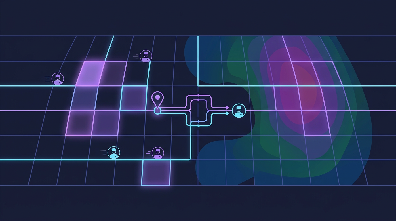
Mind Map

Ride-sharing sits at the intersection of five distinct engineering disciplines:

Geospatial indexing — finding entities by geographic proximity at millions of queries per second
Real-time streaming — continuous GPS ingestion from millions of mobile devices
Matching algorithms — assigning supply to demand under latency constraints
Dynamic pricing — algorithmic price discovery based on supply/demand imbalance
Financial transactions — pre-authorization, capture, and split payments

Most system design problems optimize one or two of these. Ride-sharing requires all five to work together coherently. By the end of this chapter you will understand the architecture behind Uber, Lyft, Grab, and DiDi, and be able to explain the geospatial indexing decision — the question that separates good candidates from great ones.

Step 1 — Requirements & Constraints

Functional Requirements

Feature	In Scope	Notes
Request a ride	Yes	Rider sets pickup and dropoff; system finds driver
Driver matching	Yes	Nearest available driver by ETA, not just distance
Real-time tracking	Yes	Rider sees driver move on map; driver sees route
Trip lifecycle management	Yes	State machine: requested → matched → en route → in-progress → completed
Fare calculation	Yes	Base fare + time + distance + surge multiplier
Surge pricing	Yes	Dynamic multiplier based on supply/demand ratio per zone
Driver location updates	Yes	Driver app sends GPS every 4 seconds
Payment processing	Yes	Pre-auth on request; capture on completion
Driver payout	Yes	Split fare: driver share after platform commission
Ride history	Yes	Rider and driver can review past trips
Ride cancellation	Yes	By rider pre-pickup or driver; cancellation fee logic
Pool / shared rides	Out of scope	Simplifies matching; add as extension
Scheduled rides	Out of scope	Focus on on-demand

Non-Functional Requirements

Property	Target	Reasoning
Matching latency	< 5 seconds from request to matched driver	User experience — longer feels broken
Location update ingestion	99.9th percentile < 500ms	GPS updates must stay fresh for matching
Driver position staleness	< 8 seconds	Two missed updates before position is stale
System availability	99.99%	Downtime = lost rides = revenue loss
Geospatial query latency	P99 < 50ms	Proximity search must not dominate matching time
Trip tracking update rate	Every 3–5 seconds on rider screen	Perceived smoothness without network overload
Payment success rate	99.95%	Failed payments require costly manual recovery
Concurrent drivers tracked	5M worldwide	Peak: urban rush hours across multiple cities

Step 2 — Capacity Estimation

Applying back-of-envelope techniques from Chapter 4 — Back-of-Envelope Estimation.

Assumptions

100 million registered riders, 5 million registered drivers
10 million rides per day (global)
1 million drivers online at peak (20% of 5M total)
Driver sends GPS update every 4 seconds while active
Average trip duration: 20 minutes
Average trip distance: 8 km

QPS Estimation

GPS updates from drivers:
  1,000,000 active drivers × (1 update / 4s) = 250,000 location updates/second

Ride requests:
  10,000,000 rides/day / 86,400s = ~116 ride requests/second
  Peak = 5× average = ~580 ride requests/second

Location queries for matching:
  Each ride request triggers ~5 proximity queries (fan-out, retry)
  580 × 5 = ~2,900 geospatial queries/second

The dominant load is location update ingestion: 250,000 writes/second. This drives the entire storage and streaming architecture.

Storage Estimation

Driver location record = 64 bytes
  (driver_id: 8B, lat: 8B, lng: 8B, heading: 4B, speed: 4B,
   timestamp: 8B, status: 4B, geohash: 12B, padding: 8B)

In-memory active driver store:
  1,000,000 drivers × 64 bytes = 64 MB   ← fits in a single Redis node

Trip records:
  1 trip = ~500 bytes (IDs, coordinates, timestamps, fare)
  10M trips/day × 500 bytes = 5 GB/day
  Annual = 5 GB × 365 = 1.825 TB/year

Location history (retained 30 days for disputes):
  250,000 updates/s × 64 bytes × 86,400s × 30 days = ~41 TB/month
  → Sample to 1 update/30s for history → 1/7.5 of full rate → ~5.5 TB/month

Bandwidth Estimation

Inbound GPS stream:
  250,000 updates/s × 64 bytes = 16 MB/s inbound

Outbound tracking to rider apps:
  10M active rides at peak × 1 update/5s × 64 bytes = 128 MB/s outbound

Summary Table

Metric	Value
Active drivers tracked	1M peak
GPS update rate	250,000 /s
Geospatial query rate	~3,000 /s
Ride request rate	~580 /s peak
In-memory driver store	~64 MB
Trip data growth	~5 GB/day
Inbound GPS bandwidth	~16 MB/s

Step 3 — High-Level Design

Key design decisions at this level:

Location Service is a write-heavy, read-heavy hot path — GPS updates land in Redis (in-memory) first, then fan out to Kafka for history persistence
Matching Service reads from Redis — geospatial proximity queries run against the in-memory store, never against disk
Ride Service owns state — the trip state machine lives in PostgreSQL; Redis holds ephemeral position data
Surge pricing is precomputed — a background job recalculates multipliers every 30 seconds per zone; Matching Service reads from a cache

Step 4 — Detailed Design

4.1 Geospatial Indexing — The Core Technical Challenge

Finding the nearest available driver is the central algorithmic problem. Three approaches dominate:

Geospatial Indexing Comparison

Approach	How It Works	Strengths	Weaknesses	Used By
Geohash	Encode lat/lng into a base32 string; nearby cells share a prefix	Simple, string-based, Redis native	Edge distortion at cell boundaries; non-uniform cell sizes	Lyft (legacy), many Redis-based systems
Quadtree	Recursively divide 2D space into four quadrants; leaves hold entities	Adaptive density — more cells in dense urban areas	Complex to implement; tree rebalancing overhead	Custom in-memory implementations
S2 Cells (Google)	Sphere projected via Hilbert curve; hierarchical cell IDs	Globally uniform area; excellent hierarchy for multi-scale	More complex than geohash; requires S2 library	Google Maps, many modern systems
H3 Hexagonal Grid (Uber)	Earth divided into hexagons at multiple resolutions	Uniform neighbor distance (hexagons touch at edges, not corners); ideal for density heatmaps	Proprietary initially; hexagons do not tile perfectly at all resolutions	Uber (production since 2018)

Recommendation for interviews: Lead with geohash (simplest to explain and reason about), then mention H3 as the production-grade alternative Uber uses. Both Redis GEOADD/GEORADIUS and S2 are worth knowing.

Geohash Deep Dive

Geohash divides the Earth into a grid. Each character added to the hash increases precision by a factor of ~32.

Precision levels:
  4 chars = ±20 km   (city level)
  5 chars = ±2.4 km  (neighborhood)
  6 chars = ±0.6 km  (block)
  7 chars = ±76 m    (building)
  8 chars = ±19 m    (precise GPS)

Example: Uber HQ, San Francisco
  Coordinates: 37.7751, -122.4193
  Geohash (6): 9q8yy9
  Geohash (7): 9q8yy9k

Proximity search using geohash:

1. Encode rider's pickup location to geohash precision 6: "9q8yy9"
2. Compute the 8 neighboring cells: "9q8yy3", "9q8yy6", "9q8yy7",
   "9q8yyd", "9q8yye", "9q8yyf", "9q8yys", "9q8yyt"
3. Query Redis: GEORADIUS or scan all 9 cells for available drivers
4. Return drivers sorted by distance

The boundary problem: A driver 100m away but in an adjacent geohash cell has a different prefix. Querying only the rider's cell misses them. Solution: always query the 9-cell neighborhood (current cell + 8 neighbors). This is standard practice.

Redis Geospatial Commands

Redis provides first-class geospatial support via its sorted set internals (geohash encoded as score):

# Driver app sends update
GEOADD drivers:available <lng> <lat> "driver_id_7831"

# Matching service finds drivers near pickup
GEORADIUS drivers:available <pickup_lng> <pickup_lat> 3 km
          ASC COUNT 20 WITHCOORD WITHDIST

# Driver goes offline or accepts ride — remove from available set
ZREM drivers:available "driver_id_7831"

Redis GEORADIUS runs in O(N+log M) where N is elements in the radius and M is total elements in the sorted set. At 1M drivers across all sets and typical urban density of a few hundred per cell, queries return in microseconds.

4.2 Driver Location Service

The Location Service is the highest-throughput component: 250,000 GPS updates per second.

Batching strategy: The Location Service does not write each GPS update individually to Redis. It batches updates in 100ms windows and uses Redis pipelines to send 25,000 updates per batch (250,000/s × 0.1s). This reduces network round-trips from 250,000/s to 10/s per Location Service instance.

Driver metadata in Redis Hash:

HSET driver:7831
    status      "available"     # available | on_trip | offline
    lat         37.7751
    lng         -122.4193
    heading     245             # degrees
    speed       28              # km/h
    updated_at  1710201600      # Unix timestamp
    vehicle     "sedan"
    rating      4.87

Stale driver detection: A background sweeper runs every 10 seconds, scanning drivers whose updated_at is more than 15 seconds old (3.75 missed updates). It sets their status to "offline" and removes them from drivers:available. This prevents matching with drivers who have lost connectivity.

4.3 Matching Algorithm

The matching algorithm finds the best available driver for a ride request. "Best" means lowest ETA to pickup, not shortest distance — a driver 2 km away in light traffic beats a driver 1.5 km away in gridlock.

Key matching decisions:

ETA over distance — OSRM (Open Source Routing Machine) or Google Maps Distance Matrix API provides driving ETAs for the top-5 candidates. Querying more than 5 is wasteful; the nearest-by-radius candidates are almost always the best by ETA too.
Sequential offer, not simultaneous — offering to multiple drivers simultaneously creates race conditions and degrades driver experience. Sequential offer with 15-second timeout is standard.
Acceptance timeout tracking — drivers who repeatedly timeout have their priority reduced in future matching rounds.

4.4 Trip State Machine

State persistence: The canonical trip state lives in PostgreSQL (trips table). Redis caches the current state for fast lookups by the tracking service. On state transition, the Ride Service writes to PostgreSQL first (durable), then updates Redis (cache).

Geofencing for DriverArrived: The system detects arrival automatically when the driver's GPS position is within 50 meters of the pickup point. This triggers an "arrived" push to the rider without the driver having to press a button — reducing driver distraction.

4.5 Real-Time Location Streaming to Rider

Once a trip is matched, the rider's app displays the driver moving on a map. This is a different problem from GPS ingestion — it is server-to-client push.

WebSocket connection management:

Each active trip maintains one WebSocket connection per rider
Connection established on trip match; torn down on trip completion or cancellation
If rider loses connection, they reconnect and get the latest cached position from Redis
See Chapter 12 — Communication Protocols for connection lifecycle details

Heading interpolation: The driver app sends position every 4 seconds, but the rider sees smooth movement. The client-side app interpolates between GPS positions using the heading and speed values, creating apparent real-time movement from 4-second samples.

4.6 Surge Pricing

Surge pricing adjusts fares upward when driver supply is insufficient to meet rider demand in a geographic zone.

Surge zones: Each city is divided into fixed geographic zones (e.g., using geohash precision 5, giving ~2.4 km × 2.4 km cells). A background service recalculates surge for each zone every 30 seconds.

Surge multiplier formula:

demand_rate     = ride_requests_in_zone / last_5_minutes
supply_rate     = available_drivers_in_zone / last_5_minutes

demand_supply_ratio = demand_rate / max(supply_rate, 1)

surge_multiplier =
    if ratio < 0.5:  1.0   (no surge — oversupplied)
    if ratio < 1.0:  1.0   (no surge — balanced)
    if ratio < 1.5:  1.2×  (light surge)
    if ratio < 2.0:  1.5×  (moderate surge)
    if ratio < 3.0:  1.8×  (high surge)
    if ratio >= 3.0: 2.0×  (cap at 2× to avoid PR issues in most markets)

Surge display UX: Before the rider confirms a surge-priced ride, the app shows the multiplier explicitly and requires confirmation. This is both a legal requirement (in many jurisdictions) and a product design pattern to manage rider expectations.

Surge decay: After supply catches up (drivers move into the zone attracted by higher fares), the surge multiplier decays on the next 30-second recalculation cycle. The system naturally self-regulates.

4.7 Fare Calculation

base_fare     = flat rate per vehicle type (e.g., $2.00 for UberX)
distance_fare = distance_km × per_km_rate (e.g., $0.90/km)
time_fare     = duration_minutes × per_min_rate (e.g., $0.15/min)
subtotal      = base_fare + distance_fare + time_fare
surge_fare    = subtotal × surge_multiplier

final_fare    = max(surge_fare, minimum_fare)  # e.g., minimum $5.00

platform_fee  = final_fare × 0.25             # 25% commission
driver_payout = final_fare - platform_fee

GPS-based metering: In-progress trip distance is computed by integrating the driver's GPS positions using the Haversine formula. This requires the location history to be reliable and low-latency — another reason GPS updates cannot be dropped during the trip.

4.8 Payment Flow

Pre-authorization strategy: The system pre-authorizes the estimated fare + 20% buffer at request time. This protects against card declines mid-trip. On completion, only the actual fare is captured; the remaining hold is released automatically.

Step 5 — Deep Dives

5.1 Handling 250,000 Location Updates Per Second

The GPS ingestion pipeline is the highest-throughput component. A naive implementation — one Redis write per GPS update — creates a write amplification problem.

Architecture for scale:

Sharding the Redis geospatial index:

A single Redis GEOADD key called drivers:available would hold 1M entries. With 250K updates/second, even Redis (capable of ~100K ops/s for simple gets) would be overwhelmed.

Solution: Shard by city or geohash prefix:

drivers:available:nyc         → New York City drivers (~50K drivers)
drivers:available:sf          → San Francisco drivers (~8K drivers)
drivers:available:la          → Los Angeles drivers (~30K drivers)
drivers:available:9q8         → Geohash prefix-based shard

Each shard fits on a dedicated Redis node. GEORADIUS queries route to the correct shard based on pickup location. With 6 shards averaging ~166K drivers each, write throughput per shard drops to ~40K updates/second — well within a single Redis node's capacity.

Kafka for durability and fanout:

GPS updates also flow to Kafka for:

Location history (Cassandra consumer) — needed for trip dispute resolution and route playback
Analytics (Spark consumer) — aggregate movement patterns for city planning, demand prediction
Surge pricing (surge calculator consumer) — real-time supply counting per zone
ETA service (traffic model consumer) — actual vs predicted travel times

5.2 ETA Estimation

ETA is displayed to the rider before matching (estimated pickup time) and during the trip (estimated arrival at dropoff).

ETA pipeline:

1. Routing engine (OSRM / Valhalla) computes base route + time
   using road network graph (OpenStreetMap or HERE Maps data)

2. Traffic layer adjusts base time:
   adjusted_eta = base_eta × traffic_factor(hour, day, segment)

   traffic_factor from:
   - Real-time GPS probe data (aggregate driver speeds per road segment)
   - Historical travel times (P50 for same segment, same hour of week)
   - Incident reports (accidents, closures) from third-party feed

3. Driver-specific adjustment:
   driver_eta = adjusted_eta × driver_speed_factor
   (derived from driver's historical on-time performance)

4. Confidence interval:
   Display range: P25–P75 of historical samples
   "Arriving in 8–12 minutes"

ETA accuracy at Uber: Uber uses deep learning models that incorporate hundreds of features (time of day, weather, day of week, local events, road segment congestion). The system achieves median ETA error of ~90 seconds for pickup ETAs. For interviews, the OSRM + traffic factor approach is sufficient.

5.3 Real-World: Uber's H3 Hexagonal Grid

Uber open-sourced H3 in 2018 as a replacement for their earlier geohash-based indexing. Understanding why illuminates the tradeoffs.

Why hexagons over squares?

Square grid: A cell has 8 neighbors.
             Corner neighbors are √2 × farther than edge neighbors.
             This creates directional bias in proximity calculations.

Hexagonal grid: A cell has exactly 6 neighbors.
                All neighbors are equidistant from the center.
                No directional bias — critical for fair surge pricing.

If surge pricing uses square zones, a driver at the corner of three zones is "closer" to two of them than the third — even if physically equidistant. Hexagonal zones eliminate this.

H3 resolution levels:

Resolution	Cell diameter	Typical use
7	~1.2 km	City-wide demand heatmaps
8	~461 m	Surge pricing zones
9	~174 m	Pickup zone precision
10	~65 m	Driver-to-rider matching
11	~24 m	Precise geofencing

H3 in driver matching at Uber:

python

import h3

# Driver sends GPS update
driver_lat, driver_lng = 37.7751, -122.4193
resolution = 9  # ~174m cells for matching

# Encode driver position
h3_cell = h3.geo_to_h3(driver_lat, driver_lng, resolution)
# → "8928308280fffff"

# Matching: find drivers in rider's cell + 1-ring neighbors
rider_cell = h3.geo_to_h3(rider_lat, rider_lng, resolution)
search_cells = h3.k_ring(rider_cell, k=1)  # center + 6 neighbors = 7 cells
# No boundary problem: hexagonal k-ring is symmetric by definition

The H3 hexagonal k-ring eliminates the 8-neighbor-query complexity of geohash and produces geometrically consistent search areas regardless of direction.

Production deployment: Uber stores H3 cell IDs as keys in Redis hashes. Each cell maps to a set of driver IDs. Updates are O(1) hash operations. The hexagonal grid also powers surge pricing heatmaps, ETAs, and demand forecasting — all on a single unified spatial index.

Architecture Diagram — Complete System

Key Takeaway

Ride-sharing is a masterclass in multi-dimensional systems design: the geospatial layer (geohash or H3) makes proximity search possible at millisecond latency; the location service must ingest 250,000+ GPS updates per second without dropping any; matching must optimize for ETA, not raw distance; and surge pricing requires a spatial aggregation pipeline that runs every 30 seconds. Any interview answer that does not address geospatial indexing, GPS update throughput, and the matching algorithm independently has missed the three core technical challenges. Uber's switch from geohash to H3 is a real-world case study in why hexagonal geometry produces fairer, more accurate proximity queries than rectangular grids.

Chapter	Relevance
Ch09 — SQL Databases	PostGIS geospatial indexing for proximity queries
Ch06 — Load Balancing	Load balancing 250K+ GPS updates/sec across location servers
Ch07 — Caching	Redis geospatial for real-time driver location lookup
Ch10 — NoSQL Databases	Time-series NoSQL for GPS event ingestion at scale

Practice Questions

Beginner

Geospatial Indexing Trade-offs: Your city deployment has a dense downtown core (50,000 drivers in 5 km²) and sparse suburbs (500 drivers in 50 km²). Fixed geohash precision 6 (~0.6 km cells) is suboptimal for both zones. Explain why, and how a quadtree adaptive index addresses the density problem at the cost of operational complexity.
Hint
In dense zones, one geohash cell contains too many drivers (slow linear scan); in sparse zones, a rider's search may return zero results and must expand to adjacent cells — a quadtree subdivides dense cells and merges sparse ones automatically.

Intermediate

Driver Matching Race Condition: A rider requests a ride. The Matching Service queries Redis and selects driver A. Before the offer is sent, a different city instance also queries Redis and also selects driver A. Both instances now try to assign driver A to different trips. Describe the race condition and design a Redis atomic solution (using SET NX or a Lua script) that prevents double-assignment.
Hint
Use `SET driver:{id}:lock {trip_id} NX EX 30` — only one instance succeeds; the other receives nil and must select the next-best available driver; release the lock after assignment confirmation or timeout.
Location Update Spike: Your Location Service normally receives 250K GPS updates/second. At 5:00 PM Friday, all 1M active drivers simultaneously accelerate and send 400K updates in one second. Your Redis pipeline batches 25K updates per 100ms window. Walk through exactly what queues fill up, what latency spikes, and how you mitigate without dropping updates.
Hint
The inbound Kafka queue absorbs the burst (backpressure); the Redis writer falls behind by one batch window (100ms lag); detect via queue depth monitoring and auto-scale the Redis writer consumer group to drain the backlog.
Surge Pricing Detection: Your surge algorithm recalculates every 30 seconds. A concert ends and 20,000 riders request rides simultaneously in a 1 km² area. The 30-second lag means thousands of bookings happen at non-surge prices. Design a system that detects demand spikes within 5 seconds and applies temporary surge, without false-surging normal traffic variation.
Hint
Maintain a sliding 5-second rolling request count per geohash cell in Redis; trigger provisional surge when the rate exceeds 3× the baseline for that cell at that time-of-week; use a hysteresis window to avoid flapping.

Advanced

Trip Dispute Resolution: A rider disputes a 15 km fare, claiming the trip was 8 km. Your Cassandra location history has GPS samples every 30 seconds (not every 4 seconds, for cost reasons). What is the maximum possible distance error from 30-second sampling at typical urban speeds (30–50 km/h)? Design a dispute resolution data model that gives customer support the tools to adjudicate accurately.
Hint
At 50 km/h, a vehicle travels 417m in 30 seconds — GPS sampling error accumulates per segment; store the raw GPS stream in a cheap cold store (S3) for dispute resolution even if the real-time pipeline uses sampled data; the dispute model should show the reconstructed path with confidence intervals.

References & Further Reading

"System Design Interview Vol 2" — Alex Xu, Chapter 13 (Proximity Service)
Uber Engineering Blog — geospatial indexing
"The Geohash Algorithm"
"RING: An Architecture for Real-Time Ride Matching" — Lyft Engineering

Part 1: Fundamentals

Part 2: Building Blocks

Part 3: Architecture & Patterns

Part 4: Case Studies

Part 5: Modern & Mastery

Chapter 22: Ride-Sharing & Geospatial Systems ​

Mind Map ​

Overview — Why Ride-Sharing Is a Landmark Interview Topic ​

Step 1 — Requirements & Constraints ​

Functional Requirements ​

Non-Functional Requirements ​

Step 2 — Capacity Estimation ​

Assumptions ​

QPS Estimation ​

Storage Estimation ​

Bandwidth Estimation ​

Summary Table ​

Step 3 — High-Level Design ​

Step 4 — Detailed Design ​

4.1 Geospatial Indexing — The Core Technical Challenge ​

Geospatial Indexing Comparison ​

Geohash Deep Dive ​

Redis Geospatial Commands ​

4.2 Driver Location Service ​

4.3 Matching Algorithm ​

4.4 Trip State Machine ​

4.5 Real-Time Location Streaming to Rider ​

4.6 Surge Pricing ​

4.7 Fare Calculation ​

4.8 Payment Flow ​

Step 5 — Deep Dives ​

5.1 Handling 250,000 Location Updates Per Second ​

5.2 ETA Estimation ​

5.3 Real-World: Uber's H3 Hexagonal Grid ​

Architecture Diagram — Complete System ​

Key Takeaway ​

Related Chapters ​

Practice Questions ​

Beginner ​

Intermediate ​

Advanced ​

References & Further Reading ​

Chapter 22: Ride-Sharing & Geospatial Systems